The essence of the Fourier transform

The content of this note reveals the questions of how and why the Fourier transform known to all power engineers works. Here we tried to refrain from using a complex conceptual apparatus, all the calculations used should be clear to anyone who has somehow mastered the initial level of the university course in higher mathematics. For all others, it is possible that the material presented is intuitive.

Currently, the Fourier transform is widely used as the basis of various tools for analyzing emergency waveforms. Examples of its use in modern waveform viewing programs:

• highlighting the effective value of the recorded electrical quantity and its current phase (Fig. 1);
• spectrum acquisition – fig. 2;
• construction of a vector diagram (Fig. 3);
• construction of temporary hodographs of complex measurements of electrical quantities (for example, resistances) – Fig. 4.

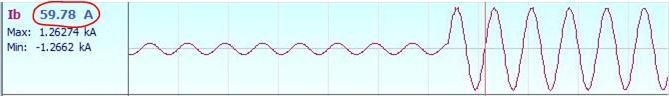
Fig. 1. Illustration of the application of the Fourier transform to extract the current value

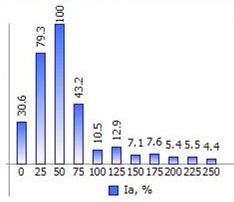
Fig. 2. Spectrum as an example of using the Fourier transform

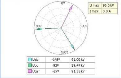
Fig. 3. Vector diagram as an example of using the Fourier transform

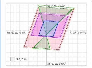
Fig. 4. Hodograph of resistance as an example of using the Fourier transform

Thus, the role of the Fourier transform in the analysis of emergency waveforms is difficult to overestimate. Next, let’s move on to its essence.

1. The Fourier transform is a certain linear operator (see Fig. 5), which converts the input signal u(t) in the time domain (t is the time) into the signal U(f) in the frequency domain (f is the frequency).

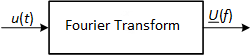
Fig. 5. Fourier transform as a “black box”

2. It is assumed that the input signal u(t) consists of a set (sum) of cosines of the following form:

where f is the frequency; A is the amplitude; φ₀ is the initial phase.

Next comes a very important statement. In accordance with the well-known Euler formula, the function cos is defined as the sum of two complex exponentials:

where is imaginary unit.

Now we can make a clarification: in the general case, the Fourier transform assumes that the input signal u (t) does not consist of a set of cosine waves, as was stated just above, but of a set of complex exponentials.

Note: in the Fourier transform, the frequency f is the frequency of the complex exponent, not the cosine.

Let us consider in more detail exactly which complex exponentials the cosine s(t) consists of. The first exponent e₁(t) describes on the complex plane the uniform motion of a point in a circle with a radius with a constant angular velocity – see Fig. 6.

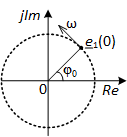
Fig. 6. The first complex exponent of which the cosine consists

The second exponent e₂(t) is the twin sister of the first exponent e₁(t), but in contrast to it, it describes the rotation of a point in a circle in the opposite direction – see Fig. 7. Also note that the graphs e₁(t) and e₂(t) are symmetrical about the real axis Re.

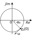Fig. 7. The second complex exponent of which the cosine consists

So, a cosine wave with frequency f consists of a complex exponent with frequency f and a complex exponent with frequency –f.

3. Periodic functions such as a sine wave, cosine wave and complex exponent have a very important property from the point of view of the Fourier transform: their average value (and the integral too) on the period is equal to zero. In other words, if we take a complex exponent with a frequency f_x and average it over a period of 1/f_x, then as a result of averaging we get a zero value. This rule is valid for almost all complex exponentials with any frequency f_x. But there is one exception to this rule. This is an exponential with a frequency f = 0 Hz, i.e. constant component. As a result of averaging the constant component over any time interval, the constant component itself is obtained, i.e. she does not reset to zero.

Let’s see how the Fourier transform is built on the rule considered.

As an example, take a cosine wave with a frequency of 50 Hz and amplitude A. We know that this cosine wave consists of two complex exponentials with frequencies -50 Hz and +50 Hz. How these components are located in the frequency domain can be seen in Fig. 8. Only two values |U(f)| nonzero – at the points of -50 Hz and +50 Hz.

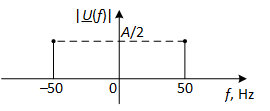
Fig. 8. View of a cosine wave with a frequency of 50 Hz and amplitude A in the frequency domain

If the Fourier transform is intended to convert the signal in the time domain u(t) to a signal in the frequency domain U(f), then in the case of the cosine wave u(t)=s(t), as U(f) we must get the function depicted in fig. 8. What can be done with s(t) to get |U(f)| as in fig. 8? For simplicity, we will not restrict ourselves to the entire function |U(f)|, but to only one of its values at f=50 Hz. At this point, the value of the function should be |U(50)|=A/2.

So, we are given the cosine s(t), the given value of the frequency f=50 Hz and information that at this frequency the equality |U(50)|=A/2 should be satisfied. How do you need to convert s(t) so that the output of the conversion is |U(50)|=A/2? Obviously, if we simply average the cosine s(t) over a period of 1/f=1/50=0.02 s, then we get zero at the output, i.e. |U(50)|=0. Therefore, simply averaging over a period is not suitable as the desired transformation. Let’s try another option. Multiply s(t) by the complex exponent with a frequency of -50 Hz:

As a result, the exponential part of the cosine s(t) with a frequency of -50 Hz turned into an exponent with a frequency of -100 Hz, and an exponent with a frequency of +50 Hz turned into a complex exponent with a frequency of 0 Hz, i.e. into the constant component. There is a frequency shift of all complex exponentials that make up the input signal by a value of -50 Hz. The way the cosine components s(t) began to settle down in the frequency domain after this (now this is the signal s₁(t)), is shown in Fig. 9.

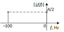
Fig. 9. View of a cosine-shifted cosine wave at -50 Hz in the frequency domain

Next, we average the received signal s₁(t) over a period of 0.02 s. As a result of averaging, the exponent included in s₁(t) with a frequency of -100 Hz () is zeroed, because the time interval of 0.02 s is equal to two of its own periods. At the same time, the second exponent with a frequency of 0 Hz, which is part of s₁(t), is not zeroed, the result of its averaging is equal . So, averaging the signal s₁(t) over a time interval of 0.02 s, we obtain

We got what we wanted, namely |U(50)|=A/2.

Actually, the Fourier transform is the two procedures considered:

1) the frequency shift of all complex exponentials that make up the input signal u(t) by –f_x so that the complex exponent with frequency f_x turns into a constant component, thereby acquiring, so to speak, immunity to zeroing by averaging.

2) averaging a signal with shifted frequencies over a time interval multiple of the periods of all complex exponentials that are part of the signal u(t) in order to zero them (all exponents, except the one that has turned into a constant component).

In the general case, the input signal u(t) includes an unlimited number of complex exponentials with all possible frequencies. In this general case, procedure 2) works only on the averaging interval from -∞ to + ∞, since only such a time interval is a multiple of any period of any complex exponent. So, we got the formula for the Fourier transform:

The above explanation of the Fourier transform helps the figurative perception of its essence. A deeper understanding of this transformation and its modifications (discrete Fourier transform, window Fourier transform, Fourier series, wavelet transform, etc.) is achieved through the concept of convolution of functions.