Kirchhoff’s laws

When calculating electrical circuits, including for modeling purposes, Kirchhoff’s laws are widely applied, which make it possible to completely determine the mode of its operation.

Before moving on to the very laws of Kirchhoff, we give a definition of the branches and nodes of an electric circuit.

A branch of an electric circuit is such a section of it that consists only of series-connected sources of EMF and resistances, along which the same current flows. An electric circuit node is a place (point) of connection of three or more branches. When going around branches connected in nodes, you can get a closed circuit of the electric circuit. Each circuit is a closed path passing through several branches, with each node in the circuit under consideration occurs no more than once [1].

The first Kirchhoff law is applied to nodes and is formulated as follows: the algebraic sum of currents in a node is zero:

∑i = 0,

or in complex form

∑I = 0.

The second Kirchhoff law is applied to the circuits of an electric circuit and is formulated as follows: in any closed circuit, the algebraic sum of the voltages at the resistances included in this circuit is equal to the algebraic sum of the EMF:

∑Z ∙ I = ∑E.

The number of equations compiled for an electric circuit according to the first Kirchhoff law is N_n – 1, where N_n is the number of nodes. The number of equations compiled for an electric circuit according to the second Kirchhoff law is N_b – N_n + 1, where N_b is the number of branches. The number of equations to be compiled according to the second Kirchhoff law is easy to determine by the type of circuit: for this it is enough to calculate the number of “windows” of the circuit, but with one clarification: it should be remembered that the circuit with the current source is not considered.

Let us describe the methodology for compiling equations according to the laws of Kirchhoff. Consider it on the example of the electrical circuit shown in Fig. 1.

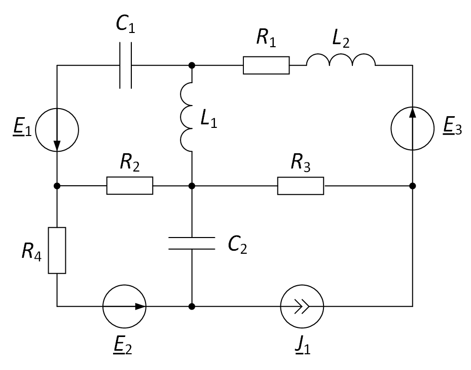
Fig. 1. Consider the electrical circuit

To begin with, you need to specify arbitrary directions of currents in the branches and specify the directions of circuit paths (Fig. 2).

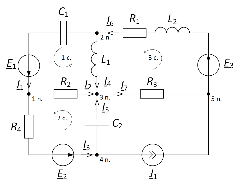
Fig. 2. Setting the direction of the currents and the direction of circuit bypass for the electrical circuit

The number of equations compiled according to the first Kirchhoff law is 5 – 1 = 4 in this case. The number of equations compiled according to the second Kirchhoff law is 3, although the “windows” in this case are 4. But we recall that the “window” containing the source current J₁ is not considered.

Compose the equations according to the first law of Kirchhoff. For this, we will take the currents “flowing” into the node with the “+” sign, and the “leaky” ones with the “-” sign. Hence, for the node “1 n.” The equation according to the first law of Kirchhoff will look like this:

I₁ – I₂ – I₃ = 0;

for the node “2 n.” the equation according to the first law of Kirchhoff will look as follows:

–I₁ – I₄ + I₆ = 0;

for the node “3 n.”:

I₂ + I₄ + I₅ – I₇ = 0;

for the node “4 n.”

I₃ – I₅ – J₁ = 0

The equation for the node “5 n.” you can not make.

We compose the equations according to the second law of Kirchhoff. In these equations, positive values for currents and EMF are selected if they coincide with the direction of the circuit. For the “1 c.” circuit, the equation according to the second Kirchhoff law will look like this:

Z_C1 ∙ I₁ + R₂ ∙ I₂ – Z_L1 ∙ I₄ = E₁;

for the “2 c.” circuit, the equation according to the second Kirchhoff law will look as follows:

-R₂ ∙ I₂ + R₄ ∙ I₃ + Z_C2 ∙ I₅ = E₂;

for the “3 c.” circuit:

Z_L1 ∙ I₄ + (Z_L2 + R₁) ∙ I₆ + R₃ ∙ I₇ = E₃,

where Z_C = – 1/(ωC), Z_L = ωL.

Thus, in order to find the required currents, it is necessary to solve the following system of equations:

In this case, it is a system of 7 equations with 7 unknowns. To solve this system of equations, it is convenient to use Matlab. To do this, imagine this system of equations in matrix form:

To solve this system of equations, we use the following script:

>> syms R1 R2 R3 R4 Zc1 Zc2 Zl1 Zl2 J1 E1 E2 E3;
>> A = [1  -1 -1    0   0        0  0;
       -1   0  0   -1   0        1  0;
        0   1  0    1   1        0 -1;
        0   0  1    0  -1        0  0;
      Zc1  R2  0 -Zl1   0        0  0;
        0 -R2 R4    0 Zc2        0  0;
        0   0  0  Zl1   0 (R1+Zl2) R3];
>> b = [0;
        0;
        0;
       J1;
       E1;
       E2;
       E3];
>> I = A\b

As a result, we obtain a column vector I of currents from seven elements, consisting of the sought currents, written in general form. We see that the Matlab software package can significantly simplify the solution of complex systems of equations compiled according to the laws of Kirchhoff.

References

1. Zeveke G.V., Ionkin P.A., Netushil A.V., Strakhov S.V. Fundamentals of circuit theory. Textbook for high schools. Ed. 4th, revised. M., “Energy”, 1975.