Loop currents method for calculating electrical circuits

When calculating electrical circuits, in addition to the Kirchhoff’s laws, the circuit current method is often used. The method of loop currents allows you to reduce the number of solvable equations.

In the method of loop currents, equations are compiled on the basis of the second Kirchhoff law, and they are equal to N_b – N_n + 1, where N_n is the number of nodes, N_b is the number of branches, i.e. the number coincides with the number of equations compiled according to the second law of Kirchhoff.

Let us describe the methodology for compiling equations by the method of contour currents. Consider it on the example of the electrical circuit shown in Fig. 1.

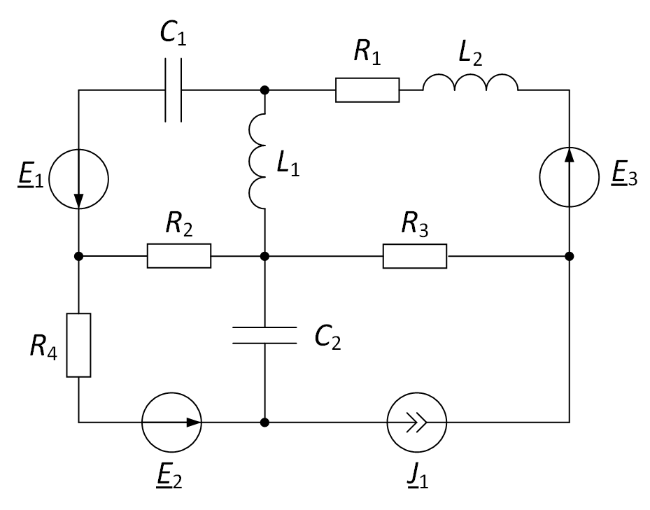
Fig. 1. Considered electrical circuit

First you need to set the direction of the circuit currents arbitrarily (Fig. 2).

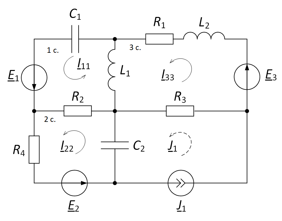
Fig. 2. The direction of the circuit currents in the electrical circuit

The number of equations compiled by the method of loop currents is 3. Here, a loop with a current source is also not considered.

We compose the equation for the circuit “1 c.”. In the “1 c.” circuit, the loop current I₁₁ flows through all the resistances R₂, Z_L1, Z_C1. In addition, the loop current of the adjacent “2 c.” circuit I₂₂ flows through the resistance R₂, and the loop currents I₁₁ and I₂₂ flow in opposite directions. A loop current I₃₃ also flows through the inductive resistance Z_L1, and the loop currents I₁₁ and I₃₃ also flow in opposite directions. When compiling the equation, you need to add up all the voltage drops (similar to Kirchhoff’s second law), while taking into account the direction of the circuit currents: if the circuit currents of adjacent circuits flow in a certain branch in one direction, then the voltage drop in this branch must be entered with a “+” sign, otherwise, with a “-” sign. The resulting amount will be equal to the sum of the EMF of this circuit, while the EMF is taken with a “+” sign if the direction of the loop current coincides with the direction of the EMF, otherwise – with a “-” sign.

Given the foregoing, the equation by the method of contour currents for the circuit “1 c.” will look like this:

(R₂ + Z_L1 + Z_C1) ∙ I₁₁ – R₂ ∙ I₂₂ – Z_L1 ∙ I₃₃ = E₁.

Similarly, we compose the equation for the contour “2 c.”. It should be noted that the equation for the circuit with the current source is not compiled, but the current from the current source must also be taken into account in the equation similarly to the loop currents of other loops. The equation itself will look like this:

–R₂ ∙ I₁₁ + (R₂ + R₄ + Z_C2) ∙ I₂₂ – Z_С2 ∙ J₁ = E₂.

For the circuit “3 c.”:

–Z_L1 ∙ I₁₁ + (R₁ + R₃ + Z_L1 + Z_L2) ∙ I₃₃ – R₃ ∙ J₁ = E₃.

In the above equations Z_C = –1/(ωC), Z_L = ωL.

Thus, in order to find the desired loop currents, it is necessary to solve the following system of equations, where the terms with the current source current are transferred to the right side of the equations:

In this case, it is a system of 3 equations with 3 unknowns. To solve this system of equations, it is convenient to use Matlab. To do this, imagine this system of equations in matrix form:

To solve this system of equations, we use the following Matlab script:

>> syms R1 R2 R3 R4 Zc1 Zc2 Zl1 Zl2 J1 E1 E2 E3;
>> A = [R2+Zl1+Zc1       -R2          -Zl1;
               -R2 R2+R4+Zc2             0;
              -Zl1         0 R1+R3+Zl1+Zl2];
>> b = [ E1;
E2 + Zc2*J1;
 E2 + R3*J1];
>> I = A\b

As a result, we obtain a column vector I of currents of three elements, consisting of the desired loop currents, where

I(1) = I₁₁, I(2) = I₂₂, I(3) = I₃₃.

Further in the diagram according to fig. 2, we arrange the directions of the currents in the branches (Fig. 3).

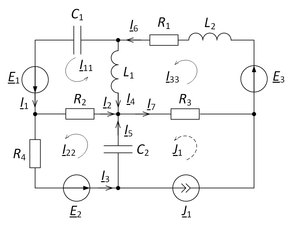
Fig. 3. Setting the direction of currents in an electric circuit

To determine the currents in the branches, it is necessary to consider all the loop currents that flow through this branch. We see that only one loop current I₁₁ passes through the branch current I₁ flows, and

I₁ = I₁₁.

Through the branch where the current I₂ flows, the loop currents I₁₁ and I₂₂ pass, and the current I₁₁ coincides with the accepted direction of the current I₂, and the current I₂₂ does not coincide. Those loop currents that coincide with the accepted direction are taken with the “+” sign, those that do not coincide with the “-” sign. From here

I₂ = I₁₁ – I₂₂.

Similarly for other branches

I₃ = I₂₂,

I₄ = –I₁₁ + I₃₃,

I₅ = I₂₂ – J₁,

I₆ = I₃₃,

I₇ = I₃₃ – J₁.

So, the method of loop currents allows you to calculate a smaller number of complex equations for calculating a similar electrical circuit in comparison with the laws of Kirchhoff.

References

1. Zeveke G.V., Ionkin P.A., Netushil A.V., Strakhov S.V. Fundamentals of circuit theory. Textbook for high schools. Ed. 4th, revised. M., “Energy”, 1975.